Apparatus Designed and Built by Physicists who have taught in the Advanced Undergraduate Lab
Torsional Oscillator
.png)
-
fully instrumented test-bed for investigating simple harmonic motion
-
variable torsion constant and rotational inertia
-
non-contact precision analog sensors provide angular position and velocity
-
damping options range from constant to velocity dependent and include a v2-friction regime
-
magnetic torque drive accommodates arbitrary drive waveforms
-
resonant behavior in time and frequency domains with "Q" ranging from less than 1 to more than 100
-
"intellectual phase space" ranges from rotational kinematics and rotational dynamics to general oscillations and waves
-
appropriate from the freshman to advanced lab, from mechanics to advanced electronics
Introduction
Simple Harmonic Oscillation Made Visible, Tangible, Accessible, Measurable
Few systems in physics have wider applicability than the Simple Harmonic Oscillator (SHO). At every level of their education, from first-year undergraduate to advanced graduate training, students will find something valuable and applicable in the physics of the Simple Harmonic Oscillator.
-
In introductory mechanics as Hooke's-Law oscillation problems;
-
In analysis of the LCR system in circuit theory;
-
In every normal-mode problem in mechanics and electromagnetism;
-
In the quantum-mechanical SHO problem in
-
one dimensional particle and molecular vibrations,
-
quantization of each mode of the electromagnetic field;
-
-
As a model for the resonant excitation of atoms or nuclei by external fields.
We have chosen a system and a set of parameters that are optimized for both seeing and learning. Quite deliberately, we have chosen a macroscopic and plainly visible mechanical system, which oscillates with periods on the order of one second so that students can see the behavior of the system on a human time scale.
We have even provided hands-on involvement. When applying a torque by fingertip students learn quite tangibly, the phase relationship required between the system's angular position and the applied torque in order to achieve resonant excitation.
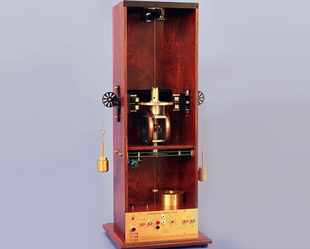
Instrument
-
The Aluminum Rotor is clamped at the midpoint of the wire and other parts are attached to it.
-
The Copper Disc both contributes to the moment of inertia and interacts with the magnetic brakes.
-
A scale on the edge of the copper disc allows visual measurement of angular deflection in radians
-
Moveable magnetic brakes on either side provide variable eddy-current magnetic damping
-
Helmholtz coils interact with a dipole mounted on the rotor both to provide magnetic torques and to measure velocity.
-
Circuit Boards mounted beneath the system provide the non-contact capacitive angular-position transducer
Motivated by the central role that the Simple Harmonic Motion plays in physics, and in physics education, TeachSpin has developed an apparatus that makes visible, tangible, accessible and MEASURABLE all the features important to the physics of Simple Harmonic Motion. Our new Torsion Oscillator was designed, from the ground up, to be a premier teaching tool for the physics of the Simple Harmonic Oscillator at every level.
An overview of the apparatus:
-
We've chosen to exploit simple harmonic motion in angle.
-
The aluminum 'rotor' structure is attached at the midpoint of a taut steel wire.
-
A copper disc, centered on the wire, is mounted on the rotor.
-
Torsional elasticity of the wire provides the 'spring constant' of the SHO.
-
Rotational inertia of the rotor and copper disc provide the 'mass' of the SHO.
-
Both the spring constant and the "mass" can be changed by the user.
-
Four wires of different diameters, and thus different torsional constants, are included. This allows the "spring constant" to be varied over an order of magnitude.
-
Extra weights, machined to produce easily calculated rotational inertia increments, are included.
-
-
Moveable magnets mounted on the wooden frame interact with the copper disc to create variable eddy-current damping.
-
Helmholtz coils are attached to the cabinet so that their axis passes both through the steel wire and through the center of a magnetic dipole system mounted on the rotor.
-
Pulleys (not shown) mount to the outside of the cabinet at the level of the copper disc.
-
Pulleys, strings, masses, and hangers are provided for static torque calibration.
Distinctive features of the Rotor System:
-
A non-contact capacitive angular-position transducer provides real-time analog angular-position information about the system to an accuracy of better than 1.0%.
-
The rotor is equipped with a 'radian protractor', allowing student calibration of the angular position sensor.
-
A real-time emf proportional to the instantaneous angular velocity of the rotor is developed by the motion of the dipole on the rotor relative to the fixed set of coils.
-
The magnet-in-coil system can be separately calibrated for sensitivity to angular velocity, and for torque per unit drive current. (In the process, students can verify the reciprocity theorem relating these two constants. They can even learn one method for the first-principles measurement of a magnetic moment.)
These features allow students to have direct access to the instantaneous 'position' and 'velocity' outputs of the system. They can view in real time (on an oscilloscope in the XY-display mode, or on a computer) the state of the oscillator in the 'phase plane'
Because we picked a mechanical system that involves no frictional or sliding contact with the rotor, our SHO corresponds to a high-Q oscillator. (In the absence of deliberate damping, our Torsional Oscillator displays a Q of over 100.)
Three independent damping systems:
Students can investigate the various transient or driven responses of the oscillator to each of the three available damping systems.
-
Eddy-current magnetic-damping 'brakes' provide a damping force that's linear in velocity. This damping is adjustable in magnitude, from negligible to beyond-criticaldamping;
-
Damping by sliding friction yields a damping force that's independent of the velocity's magnitude;
-
Paddles-on-arms can be easily attached allowing investigation of fluid damping by air which gives a damping force approximately quadratic in velocity.
Helmholtz Coil/Dipole Modes of operation set from electronics box:
-
Toggle set to Velocity Readout gives angular velocity.
-
Toggle set to Coil Drive allows external drive by arbitraryanalog electrical
waveforms.


Experiments
Simple Harmonic Oscillation Made Visible, Tangible, Accessible, Measurable
Here is an instrument whose wide "intellectual phase space" invites an exceptionally wide variety of experiments at an equally wide variation of levels. The almost embarrassingly perfect data reassures students that even the most counter-intuitive data is correct. (On the linear plots, R2 value results are included to indicate just how closely the measurements match the plotted line.)
Most probably, the "Experiments" section of the Torsional Oscillator will always be a work in progress. This apparatus has such a wide range of possible experiments that we expect to be "playing" with it and adding experiments for some time to come. The graphs posted below include explorations of the apparatus itself as well as investigations of simple harmonic oscillations.
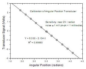
Getting Started - Calibrating the Angular Position Transducer
Students can begin their exploration by calibrating the angular position transducer. The graph shown plots the transducer output voltage as a function of the angular position when the position is in radians.
The scale along the edge of the copper disc is marked off with 0.2 radians per major division and 0.02 radians per minor division. The angular position is read by reference to a sighting line (not shown in the picture) which is mounted on a plastic arm which extends at the front of the apparatus. For the apparatus used to take this data, the graph indicates that the 3.0 radian marker is close to the sighting line when the transducer voltage is 0. (In the process of calibrating this apparatus, students also become adept at the combination of care and estimation required when working with real data.)
Finding k, the "Spring Constant" of the fiber
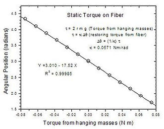
Static Measurement of the Spring Constant
The apparatus comes with two low friction pulleys which mount on supports located on the outside of the case. Strings wrapped around the rotor shaft go over the pulleys and masses can be loaded onto the attached hangers in increments of 50 grams. The strings and pulleys can be arranged to create either counter-clockwise (+) or clockwise (-) torques. To prevent unbalanced forces on the rotor, weights of equal mass are placed on both sides of the apparatus. As can be seen from the both the obvious fit of the points on the graph and the R2 value, the relationship between angle and torque is remarkably linear, making this an ideal system for exploring simple harmonic motion.
Dynamic Measurement of the Spring Constant and Moment of Inertia
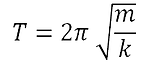
Students can also use the harmonic oscillation of the torsional oscillator to find both the spring constant of the wire and the moment of inertia, , of the rotor/copper disc system. Most students are familiar with the standard spring equation:
For the Torsional pendulum, this becomes:

where gives the rotational inertia of the system with the addition of n extra masses. The apparatus comes with a set of eight precisely machined masses which can be attached to the copper disc to vary the moment of inertia of the system. Each mass is a quarter circle arc of known inner and outer radius. The calculation of the additional moment of inertia, ΔI, provided by each mass is a good exercise in finding the moment of inertia of an extended mass. A bit of integration gives:


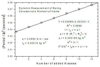
To keep the system in balance, the masses are added in pairs on either side of the disc. Some algebraic manipulation of the equation for T yields the expression on the graph below, which shows why plotting against the number of added masses gives a straight line. This graph was created using measured values of the period of torsional oscillation taken with the prototype instrument. (For the production version, different masses have been used so this data will not be numerically equal to that taken by students.) The slope of the graph gives the torsional constant of the wire. From the Y intercept, (the moment of inertia of the system with no added masses) can be determined. This moment of inertia of the rotor system can be compared with a value computed (using the dimensions and density of the copper disc) for the copper disc only. It will be interesting for students to note that the copper disc accounts for a very large portion of the moment of inertia.
Applying Static Torque Magnetically
TeachSpin's Torsional Oscillator represents a resonant system that can be excited by arbitrary drive waveforms, and these are applied as currents in a drive coil which interacts with a permanent magnet on the rotor. It is straightforward to send a steady current into the rotor, and to see how the rotor deflects to a new equilibrium position. The data in the graph to the right shows, however, that the response is not linear in the current.
From this graph, of Angular Deflection as a function of Coil Current, it is immediately obvious that using the current as an indicator of the torque driving the system will be valid only for small amplitude oscillations.
And that is the way it should be! After all, the torque you get is, in fact, a cross product between the magnetic moment of the magnets mounted on the rotor, and the magnetic field of the coils. The field of the coils is certainly linear in the current. The torque, however, is a cross product which depends not only on the magnetic moment and magnetic field, but also on the sine of the angle between the magnetic axis and the coil axis. Those axes start out nearly perpendicular, but as the rotor turns, the sine factor drops well below one. If we make a correction for this angular factor, we do find a signal that is wonderfully linear in the coil The resulting graph has a slope which is jointly due to the magnetic moment 'µ' of the permanent magnet, and the field per unit current that the coil generates. Since that coil constant 'k' can be computed from the coil geometry, this result also provides a way to measure the magnetic moment of the permanent magnet, and in SI units too -- this is 'torque magnetometry' in action.

Damped Oscillations
Eddy Current Damping
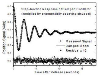
The eddy-current damping in the Torsional Oscillator depends on currents induced in the copper disk of the rotor by stationary permanent magnets. These magnet structures can be adjusted in position to change the damping of the system from nearly zero all the way to, and beyond, critical damping.
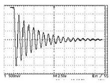
Said another way, the 'Q' of the oscillator system can be varied from under 0.5 to over 100. For any chosen value of damping, the system acts like a textbook example of the damped simple harmonic oscillator. The graph shows the angular-position signal, as a function of time, for the rotor released from rest. The data for Eddy Current Damping fit the textbook form of an exponentially-decaying sinusoid to terrific precision, so we've shown the 'residuals', or data values minus the best-fit model, multiplied by 10-fold, to display the quality of the fit.
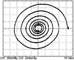
Relating Angular Position and Angular Velocity - the "Death Spiral"
The coil/magnet system can be used reciprocally, as a 'generator' instead of a 'motor'. In this mode, you disconnect the current supply, and attach a voltage recorder to the coils; now, any angular velocity of the rotor moves the magnet within the coils, and thus generates a measurable emf. The coil can then be used as an angular velocity transducer.
Because our transducers allow us to convert both angular position and angular velocity into voltages, we can compare the two in real time and examine the interesting patterns that result. To create the trace below, we used the oscilloscope in the x-y mode with the angular position signal on the x-axis and angular velocity signal on the y-axis. The rotor was turned away from its equilibrium position and then released. Students will enjoy exploring the way varying the damping affects the shape of the "death spiral."
Angular Position versus Time for Three Types of Damping
The Torsional Oscillator is intrinsically a low-loss system, since there is no sliding or frictional contact anywhere in its mechanism. But we've included provision for adding any of three forms of deliberate damping. These represent sliding-friction or Coulomb damping; eddy-current damping; and fluid-drag damping. The three forms can be modeled as giving v0, v1, and near-v2 damping forces, where v is a relevant linear velocity.
Motion of the oscillator, when released from a non-equilibrium position, depends a great deal on which form of damping is chosen. The data below show that decaying oscillations, obtained under these three forms of damping, are very different in character.

Coulomb Damping, or v0 Sliding Friction, of tensioned strings on hub (note linear envelope)
Magnetic Eddy Current or v1 Damping (note exponential envelope)

Fluid-Drag Damping, showing approximately v2 dependence created by air on paddles
Driven Oscillations
The methods discussed so far give you, as investigator, a harmonic-oscillator system that is fully characterized, for inertia, damping, restoring force, and sensitivity to torque; better still, they give you a way to inject any torque waveform you wish into the system.
Steady State Response to a Sinusoidal Drive
You can discover for yourself the special role of sinusoidal drives (only for sinusoidal drive will the response, in general, be sinusoidal), but you can also inject any other waveform you wish -- triangle waves, pulses, square waves, even noise waveforms.
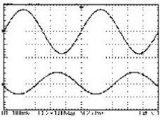
For the special case of sinusoidal drive, you can see that the response, in steady state, will be at the same frequency as the drive, but shifted in phase. In the oscilloscope screen capture at the right, the Upper Trace shows the waveform of the applied drive coil, and the Lower Trace shows the angular-position signal of the steady state response.
Only at very low frequencies will these waveforms be 'in phase', and as you approach the condition of resonance, these waveforms will get to be 90 degrees out of phase.
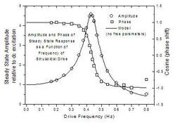
Finding the "Transfer Function" of the Oscillator System
Once you can measure the response, in amplitude and phase, to a sinusoidal drive, you can repeat this measurement over a range of frequencies to acquire the 'transfer function' of the oscillator system.
The data obtained (for one setting of the eddy-current damping strength) is shown in amplitude, and in phase shift.
Of course the transfer function can be predicted theoretically for this example of a 'linear time-invariant system', and the graph above shows the theoretical curves underlying the data points. But the theory included above is NOT a best fit; instead, it is a prediction, with no free parameters, based on prior measurements of the system, such as damped oscillatory decay and the response to static torques.