
Apparatus Designed and Built by Physicists who have taught in the Advanced Undergraduate Lab
Noise Fundamentals

-
Detect and quantify Johnson noise, the ‘Brownian motion’ of electrons
-
Deduce Boltzmann’s constant, kB, from the temperature dependence of Johnson Noise
-
Observe and quantify shot noise in order to measure the fundamental charge ‘e’
-
Configure front-end low-level electronics for a variety of measurements
-
Investigate ‘power spectral density’ and ‘voltage noise density’ of signals, and their V²/Hz and V/√Hz units
-
Apply Fourier methods to digitally process noise signals into noise densities
-
Explore amplification, filtering-in-frequency, squaring, and averaging-in-time
-
Develop skills applicable across the breadth of measurement science
Introduction
TeachSpin's Noise Fundamentals is a set of tools for teaching and learning about electronic noise in the advanced and intermediate laboratory. The noise present in all electronic signals limits the sensitivity of many measurements. That, in itself, would be reason enough to motivate learning how noise can be quantified. But electronic noise can be much more than a nuisance, or a limit -- in the famous phrase of Landauer, sometimes ‘noise is the signal’. In fact, there are at least two cases in which the measurement of noise can give the values of fundamental constants.
By concentrating on the processing and measurement of Johnson noise and shot noise, TeachSpin’s Noise Fundamentals allows students to determine both Boltzmann’s constant, kB, and the magnitude of the charge on the electron, ‘e’.d
Johnson noise is the fluctuating emf which arises spontaneously in any resistor at absolute temperature T > 0. Nyquist’s prediction is that the mean square of this emf obeys
< V (t)² > = 4 k T (R/B) ⌂f,
where ⌂f is the bandwidth over which noise is measured. This result allows Boltzmann’s constant kB to be measured.
Shot noise is a measure of the fluctuations observed in certain currents, due to the granularity imposed on them by the quantization of charge. In this case, Schott’s prediction is that a dc current i dc will be accompanied by fluctuations obeying another mean-square relation,
< [δi(t)] > = 2 2 e i ⌂f dc
This result allows the magnitude of the fundamental charge e to be measured.
Noise from either of these sources, and many more, can be observed because of the modular, and user-configurable, arrangement of our electronics. The transparent signal-flow layout of our apparatus makes it very clear how noise is quantified in practice, since the processes of amplification, filtering-in-frequency, squaring, and averaging-in-time can be understood separately and in detail. The result is a method for quantifying noise, and noise densities, that students can actually understand. This generates a portable set of skills applicable across the breadth of measurement science.
Noise measurements have a very current application in many areas of physics. Review this recent Colloquium Announcement from University at Buffalo Physics Department (Dr. Reichert's university). This colloquium discussed noise measurements that help characterize electron and hole spin fluctuations in semiconductiors. Noise is a neglected topic in our undergraduate programs, but that can be ameliorated with the adoption of Noise Fundamentals (NF1-A) into your laboratory curriculum.
Instrument
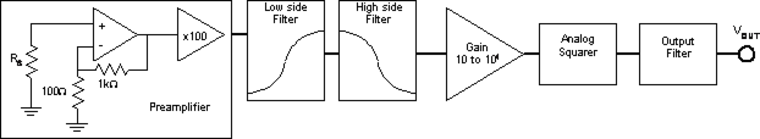
TeachSpin’s Noise Fundamentals apparatus allows students to investigate many aspects of electronic noise measurement. The apparatus consists of several parts: a clear dewar mounted on an adjustable-height wooden support; a temperature module with a thermal probe into which a variety of samples can be mounted; a high-level electronics controller with individually accessible modules; and a low-level electronics controller which students will open to reconfigure the preamp. The block diagram below gives an overview of the process.
Several experiments require students to open the electronics box, examine the circuit board and both select and install appropriate components needed to make their measurements. As is characteristic of all TeachSpin experiments, the apparatus is robust enough to allow students to make and correct a wide variety of “mistakes” without damaging the instrument. And it is this ability to explore with confidence that gives students not only ownership of a particular measurement, but also a taste of the satisfaction of experimental exploration.
The traditional TeachSpin wooden case houses the High-Level Electronics, which contains two filtering modules (to define noise bandwidth), a main-amplifier section (to give adequate gain), an analog-multiplier section (to perform the necessary squaring operation), and, finally. a time-averager (to complete the ‘mean square’ operation essential to the quantification of noise).
Also in the photograph are two user-supplied components needed to complete the necessary diagnostics and measurement capability: a digital multimeter and an oscilloscope. Not shown are the ‘parts bins’, containing all the electronic parts, tools, and cables useful for configuring this versatile apparatus into the form required for a wide variety of projects.


The Low-Level Electronics contains some utility functions (above left) and two Modules. At the upper left, you see the Thermal Control module, for interfacing to the Probe. In it are a voltage supply (for the heater which raises the probe’s temperature above 77 K) and a current supply (for powering the transdiode temperature transducer in the probe).
At the upper right in the photograph is the Pre-amplifier, the front-end electronics for all noise measurements. Front-panel controls supplement internal user-chosen configurations to make this a very versatile first stage in the measurement of various kinds of noise.
At the bottom, you see provision for Signal Attenuation (used in optional calibration activities) and a utility Series Resistance. Also visible are two low-noise power supplies, which are used for various biasing and energizing tasks. Additional low-noise power supplies energize all the circuits in the low-level electronics – no batteries are required.
The entire front panel of the low-level electronics is readily removed from its metal case, allowing easy access to the interior for user re-configuration. In this view, the Pre-amp section is at the lower right, and the screw-terminal blocks can be seen. These allow the re-wiring (without soldering!) of the front end. Students can create inverting and non-inverting amplifiers, or a current-to-voltage converter. Even the front-end operational-amplifier chip is easily exchanged or replaced.
In this view, the Temperature Control electronics are at lower right. They too allow reconfiguration via terminal blocks. In particular, users have full control over the leads headed down into the thermal probe.
At the upper right is a heavily-shielded aluminum ‘bathtub’ in which the input power for the whole box is conditioned for low noise. Across the top is the board supporting the utility functions within the low-level electronics. Here too, terminal blocks allow maximum flexibility of use of present (and future!) front-panel modules.

The High-Level Electronics are also organized into modular form, to be flexibly interconnected by the user with the cables supplied. Here you can see the two frequency-filtering modules (which specify the bandwidth of noise to be quantified), a variable-gain main amplifier module, and the multiplier module (typically used to execute the squaring function). Here also is the output section which performs the time average, runs the display meter, and sends a voltage to a user-supplied digital multimeter or other d.c. voltage-measuring device.
Not shown in this view is a rear-panel Noise Calibrator, a source of fixed-power, fixed-bandwidth, and accurately-quantifiable pseudo-noise. This provides an optional reality check for students learning to quantify noise.
Power to the entire chain of electronics is supplied by a universal power supply, mounted remotely in the supply cord to the high-level electronics. All the issues of power conditioning and ground-referencing have been handled, so our system is ready to use, without tears.
Experiments
Noise Quantification
Noise describes an electronic signal which has zero mean value and random time variation, yet with stable statistical properties. But how is noise actually measured? How can we turn a signal that is ac and contains all frequencies into a single, measurable, number?
The noise voltages which students will manipulate in this apparatus are systematically quantified by an actual all-analog re-creation of the theoretical mean-square definition of noise. Students configure the apparatus so that a tiny noise voltage V(t) is:
* pre-amplified, by a gain factor G1
* filtered, in frequency space, by a filter function G(f), typically used to define lower and upper bounds to the spectrum
* further amplified by a user-chosen gain factor G2
* squared by a real-time analog multiplier
* and, finally, time-averaged over a user-chosen averaging time.
The whole process results in a nearly steady d.c. voltage which is easily measured by a multi-meter attached to the output connector of the high-level electronics box. It is this voltage that is related, by known coefficients, to the crucial ‘mean square noise’ <V(t) >. Here, writing the quantity as <brackets> indicates that it represents a time average. The filter function, G(f), defines the ‘effective noise bandwidth’ Δf, which appears in theoretical predictions of the statistical properties of noise.
Johnson Noise
Our unit is shipped to allow immediate out-of-the-box measurement of Johnson noise. This noise source arises as a spontaneously-appearing and fluctuating emf, VJ(t), across any resistor or dissipative electrical element. A famous theory of Nyquist claims that the size of this noise is given by
< [VJ(t)] > = 4 k T R ⌂f.
In our apparatus, students can measure the left-hand-side via the actual mean-square definition, and test the predicted dependence on
* source resistance R, from 10Ω to 100 MΩ
* source temperature T, from 77 K to 400 K
* bandwidth Df, variable in width and location in frequency space, up to frequency 100 kHz
With these three tests performed, students can then extract a measured value of kB, Boltzmann’s constant.
Shot Noise
Another very important form of electronic noise is shot noise, which arises because (some) electric currents are subject to fluctuations due to the quantization of charge. In fact, for any current consisting of the statistically-independent arrivals of electrons, each of charge –e, constituting collectively an average current of i , the instantaneous current i(t) = i + δi(t) has fluctuations, of a size first predicted by Schottky as:
< [δi(t)] > = 2 e i ⌂f.
In our apparatus, the simplest shot-noise source is the photocurrent produced when a p-n junction photodiode is illuminated by an incandescent bulb. Installing this assembly within the pre-amp, and re-configuring the front end to be a current-to-voltage converter, students can translate the current fluctuations into a measured mean-square voltage noise. They can test the predicted variation of current fluctuations:
-
over a range of dc currents i from <10 nA to >100 μA
-
and for bandwidths ⌂f varying in width and location in frequency space.
With those i and ⌂f dependencies verified, students can harvest an all-electronic measurement of the fundamental charge e. Precisions of order 1%, and accuracies of a few per cent, are available with the apparatus as-is, and the accuracy can be improved to 1-2% by attention to various calibration tasks.
What’s more, students can verify that not all currents are subject to shot noise of this form, by showing that alternative sources of dc current display fluctuations much smaller than those predicted by the formula above. In fact, the reconfigurable front end allows the exploration of shot-noise-limited, and sub-shot-noise, currents, from sources dependent on, and independent of, the photoelectric effect.
Calibrations
We have deliberately structured the low-level and high-level electronics to allow full user calibration of every factor involved in experimental noise measurements.
In the as-supplied condition, the pre-amp and main-amp gains G1 and G2 can be trusted to better than 1% over the relevant bandwidths. The filter sections give bandwidths defined to better than 2% as supplied, and simple calibrations can reduce this to <1% uncertainty. What’s more, we’ve chosen circuits with good high-frequency behavior, so their performance in the relevant dc-to-100 kHz band can be trusted in detail. The result is that interested students can pursue statistical, and systematic, errors in this apparatus, at a level of 1%, with confidence.
The built-in Noise Calibrator supplies pseudo-random noise, uniform in density in the
0-32 kHz hand, with output of rms measure near 212 milliVolts. Students will learn how this gives a ‘noise power density’ near 1.40 x 10⁻⁶ V2/Hz, and will also learn why this entails a ‘voltage noise density’ near 1.19 mV/ √Hz, milliVolts per root Hertz, in this band.
The Manual also has an Appendix giving the details of how an amplified (but not squared) noise signal can be digitized (say, with a digital ‘scope) and processed (on a computer) to give a Fourier –spectrum view of noise, and noise density. Students can learn to do what ‘scopes’ FFT functions typically will not do: create spectral-density graphs whose vertical axes are properly calibrated in V2/Hz or V/√Hz units.
Projects
We’ve designed our system for maximum versatility. The low-level electronics can be re-configured; the high-level electronics can be re-cabled. Our manual suggest many projects branching out of noise quantification, which permit investigations much broader than a search fixated on numerical values for kB and e. Beginning students will learn just what to do, but advanced students can indulge their creativity, with our Noise Fundamental apparatus. (See Noise Fundamentals - Annotated Table of Contents)
Additional Resources
Specifications
Accessories
Pre-amplifier module user-configurable; as shipped, first stage is FET-input operational amplifier, non-inverting mode, gain G1 = 600, -3 dB bandwidth > 1.0 MHz, input impedance > 100 MΩ
Temperature module with current source, accuracy <1%, 10 nA to 1 mA; heater voltage supply 0 - 25 V (for floating loads), 330 mA current capability
High-level Electronics filter sections are state-variable 2-pole Butterworth design; main amplifier gain G2 adjustable from 10 to 104, -3 dB bandwidth > 1.4 MHz
Noise Calibrator output level ≈ 212 ± 2 mV, rms measure, located >99% in 0 < f < 32 kHz range, with spectral density uniform to ± 2%.
Noise Fundamentals requires the use of a digital storage oscilloscope, a digital multimeter, and the use of liquid nitrogen for explorations in temperature. Certain calibration exercises also require the use of a sine/square waveform generator.
The instrument comes supplied with all other required apparatus, including all the samples, cables, replacement parts, and tools required for all of the projects described in the Manual.